机器学习平凡之路三

机器学习平凡之路三

1. 线性回归

网店销售额预测

步骤说明

1. 明确定义所解决的问题——网店销售额的预测

2. 数据收集和预处理环节分5步走

   1. 收集数据
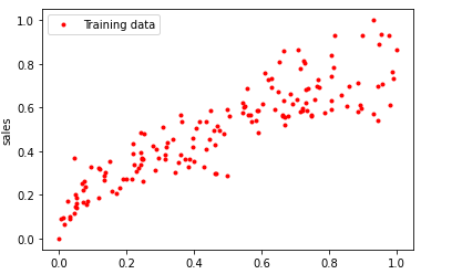
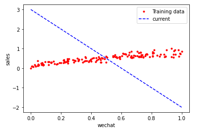
   2. 收集的数据可视化，熟悉数据的结构
   3. 做特征工程，使数据更好的被机器识别
   4. 查分数据集为训练集和测试集
   5. 做特征缩放，把数据压缩到比较小的区间中

3. 选择合适的机器学习算法

   1. 确定机器学习的算法(线性回归算法)
   2. 确定线性回归的假设函数
   3. 确定线性回归的损失函数

4. 通过梯度下降训练机器，确定内部参数的过程

5. 进行超参数调试和性能优化

简明的说就是发现一个能有此到彼的函数，如果函数只包括一个自变量和一个因变量，这个就是一元线性回归。包含2个以上的自变量就是多元线性回归

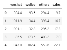
步骤一数据读取和可视化

import numpy as np
import pandas as pd
df_ads = pd.read_csv('advertising.csv')
df_ads.head()

步骤二数据的相关分析

import matplotlib.pyplot as plt
import seaborn as sns
sns.heatmap(df_ads.corr(),cmap='YlGnBu',annot=True)
plt.show()

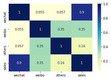
通过相关系分析，可以得知销售额和通过微信投入的是最有效地正比

sns.pairplot(df_ads,
            x_vars =['wechat','weibo','others'],
            y_vars ='sales',
            height=4, aspect=1,kind='scatter'
            )

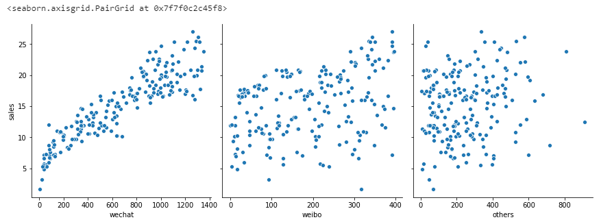
步骤三数据集清洗和规范化

上面的图可以发现微信广告的投入和销售额的相关性比较高，所以就只保留微信投入和销售金额

X = np.array(df_ads.wechat) # 构建特征集。
y = np.array(df_ads.sales) # 构建标签集
print(X.ndim)
print(X.shape)
print(X)

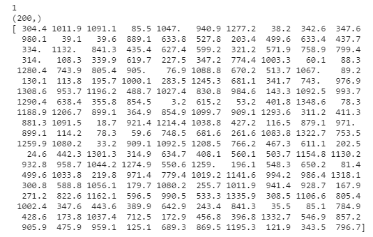
对于回归问题的数值类型数据集，机器学习模型读入的规范格式应该是2D张量.形状为(样本数,标签数)

步骤三拆分变形后的数据集

X = X.reshape(len(x),1)
y = y.reshape(len(y),1) # 对特征及和标签集进行变形
from sklearn.model_selection import train_test_split
X_train,X_test,y_train,y_test = train_test_split(X,y,
                                                test_size=0.2, random_state=0) # 拆分数据集

步骤四数据归一化

归一化，相当于数据的分布不变，但是值都落入一个小的特定区间。

常见的一个归一化公式如下 x = x-min(x) / max(x)-min(x)

'''from sklearn import preprocessing
min_max_scaler = preprocessing.MinMaxScaler()#默认为范围0~1，拷贝操作
#min_max_scaler = preprocessing.MinMaxScaler(feature_range = (1,3),copy = False)#范围改为1~3，对原数组操作
x_minmax = min_max_scaler.fit_transform(x)'''

# 1表示横轴，方向从左到右；0表示纵轴，方向从上到下。当axis=1时，数组的变化是横向的，而体现出来的是列的增加或者减少。
# 自行定义一个
def scaler(train,test):
    min = train.min(axis=0)
    max = train.max(axis=0)
    gap = max-min
    train -= min
    train /= gap
    test -=min
    test /= gap
    return train, test
X_train, X_test = scaler(X_train, X_test)
y_train, y_test = scaler(y_train, y_test)
plt.plot(X_train,y_train,'r.',label ='Training data')
plt.xlabel('wechat')
plt.ylabel('sales')
plt.legend()
plt.show()

步骤五选择合适的机器学习模型

1. 确定选用什么类型的模型
2. 确定模型的具体参数

说明

y = ax+b （a代表直线的斜率,b是截距也就是与y轴相交的位置）

y = wx+b (w替换成a代表权重,参数b称作为偏置)

假设函数

y-hat = wx+b

h(x) = wx+b (h(x)就是假设函数,也可以叫做预测函数)

机器学习的目标就是确定假设函数h(x)同时也是在确定w和b

损失函数

比如一个模型3x+5和100x+1,哪一个更好，损失是对糟糕预测的惩罚。损失也是误差，也称作成本或代价，也就是当前预测值和真实值之间的差距体现。因为每一组不同的参数，机器会针对样本数据集算一次平均损失，计算平均损失是每一个机器学习的必要环节

损失函数的表现形式为L(w,b)

损失函数一般有 L2损失函数，L1损失函数,平均偏差误差函数 (回归)

交叉熵损失函数,多类SVM损失函数(分类)

均方误差函数的实现过程:

1. 对于每一个样本y-yhat,这是预测值和真实值的差异，但损失值与参数w和b有关
2. 将损失值进行平方，平方后都变为正数，这个值叫做单个样本的平方损失
3. 所有平方损失相加，根据数量求平均值。

# 定义损失函数
def loss_function(X,y,weight,bias):
    y_hat =weight*X + bias
    loss = y_hat-y
    cost =np.sum(loss**2)/2*len(X) # 这里2相当于去抵消平方后的产生的洗漱
    return cost
print(loss_function(X_train,y_train,weight=5,bias=3))
print(loss_function(X_train,y_train,weight=100,bias=1)) # 系数越小也合适

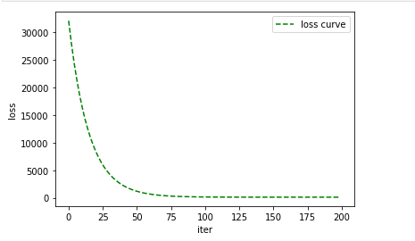
通过梯度下降找到最佳参数

训练机器，成为拟合的过程。为了确定内部的w和b。怎么才知道他们的最佳值了。最无脑的方式就是，随其生成1万个w和b的不同组合。然后挨个计算。确定一万种最优的。不过最好的理想结果是每做一次都更接近真相。也就是最精髓的梯度下降

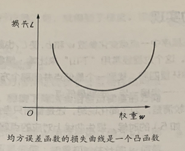
通过凸函数确保有最小损失点。比如L和W单独看。

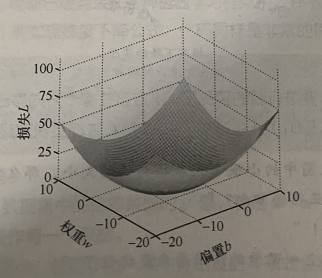
w和b共同作用

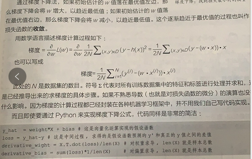
关于梯度下降的实现

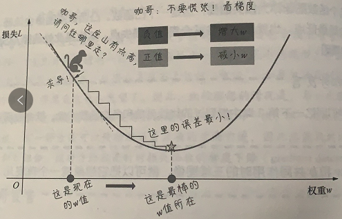
通过导数，描述函数在某点附近的变化率。求导后为梯度为正值。说明L随着W的增大而增大，反之减小

梯度具有两个特征也就是方向和大小，通过梯度下降法会沿着负梯度方向走一步，以降低损失

关于学习速率

求导知道了后，接下来是学习速率，也就alpha

梯度下降实现

def gradient_descent(X,y,w,b,lr,iter):
    l_history = np.zeros(iter)
    w_history = np.zeros(iter)
    b_history = np.zeros(iter)
    for i in rang(iter):
        y_hat = w*x+b
        loss = y_hat-y
        deruvative_w = X.T.dot(loss)/len(x) # 权重求导
        deruvative_b = sum(loss)*1/len(x)
        w = w - lr*deruvative_w
        b = b - lr*deruvative_b
        l_history[i] = loss_fuction(X,y,w,b)
        w_history[i] = w
        b_history[i] = b
    return l_history,w_history,b_history

实现线性回归并调试参数

iterations = 100
alpha =1
weight =-5
bias =3
print('损失值:',loss_function(X_train,y_train,weight,bias))
plt.plot(X_train,y_train,'r.',label='Training data')
line_X  = np.linspace(X_train.min(),X_train.max(),500)
line_y = [weight*xx + bias for xx in line_X]
plt.plot(line_X,line_y,'b--',label='current')
plt.xlabel('wechat')
plt.ylabel('sales')
plt.legend()
plt.show()

调整学习速率

如果损失函数和求导过程没有出现错误,一般造成损失过大的在于学习速率

通过比较学习速率和迭代次，选择最优

loss_history,weight_history,bias_history = gradient_descent(X_train,y_train,weight,bias,alpha,iterations)
plt.plot(loss_history,'g--',label='loss curve')
plt.xlabel('iter')
plt.ylabel('loss')
plt.legend()
plt.show()  # 学习

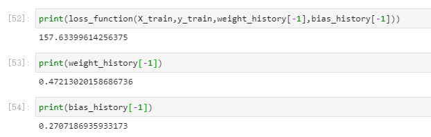
做完这一切也就是找到了最佳的两个参数

关于多元线性回归基于以上的同等道理

下面贴出代码如下:

import numpy as np # 导入NumPy数学工具箱
import pandas as pd # 导入Pandas数据处理工具箱
from keras.datasets import boston_housing #从Keras中导入mnist数据集
#读入训练集和测试集
(X_train, y_train), (X_test, y_test) = boston_housing.load_data()

def cost_function(X, y, W): # 手工定义一个MSE均方误差函数，W此时是一个向量
# X -> 是一个矩阵，形状是(N,4),N是数据集大小，4是特征数量
# W -> 是一个向量，形状是(4,1)（1*）
#   y_hat = X.dot(weight) # 这是假设函数,其中已经应用了Python的广播功能
#   y_hat = np.dot(X,weight) # 也是正确的
    y_hat = X.dot(W.T) # 也是正确的 点积运算 h(x)=w_0*x_0 + w_1*x_1 + w_2*x_2 + w_3*x_3    
#   y_hat = np.dot(X,weight.T) # 也是正确的
#   y_hat = weight.dot(X) # 错误 shapes (4,) and (160,4) not aligned: 4 (dim 0) != 160 (dim 0)
#   y_hat = np.dot(weight,X) # 错误 shapes (4,) and (160,4) not aligned: 4 (dim 0) != 160 (dim 0)
    loss = y_hat-y # 求出每一个y’和训练集中真实的y之间的差异 
    cost = np.sum(loss**2)/len(X) # 这是均方误差函数的代码实现
    return cost # 返回当前模型的均方误差值

def gradient_descent(X, y, W, lr, iter): # 定义梯度下降函数
    l_history = np.zeros(iter) # 初始化记录梯度下降过程中损失的数组
    W_history = np.zeros((iter,len(W))) # 初始化权重数组 
    for iter in range(iter): # 进行梯度下降的迭代，就是下多少级台阶
        y_hat = X.dot(W) # 这个是向量化运行实现的假设函数   
        loss = y_hat-y # 中间过程, y_hat和y真值的差
        derivative_W = X.T.dot(loss)/(2*len(X)) #求出多项式的梯度向量
        derivative_W = derivative_W.reshape(len(W)) 
        W = W - alpha*derivative_W # 结合下降速率更新权重
        l_history[iter] = cost_function(X, y, W) # 损失的历史记录 
        W_history[iter] = W # 梯度下降过程中权重的历史记录
    return l_history, W_history # 返回梯度下降过程数据
    
#首先确定参数的初始值
iterations = 12000; # 迭代12000次
alpha = 0.00001; #学习速率设为0.00001
weight = np.array([0.5,1.2,0.1,0.1,0.1,0.1,0.1,0.1,0.1,0.1,0.1,0.1,0.1]) # 权重向量
#计算一下初始值的损失
print ('当前损失：',cost_function(X_train, y_train, weight))

# 定义线性回归模型
def linear_regression(X, y, weight, alpha, iterations): 
    loss_history, weight_history = gradient_descent(X, y, 
                                                    weight, 
                                                    alpha, 
                                                    iterations)
    print("训练最终损失:", loss_history[-1]) # 打印最终损失
    y_pred = X.dot(weight_history[-1]) # 预测
    traning_acc = 100 - np.mean(np.abs(y_pred - y)/y)*100 # 计算准确率
    print("线性回归训练准确率: {:.2f}%".format(traning_acc))  # 打印准确率
    return loss_history, weight_history # 返回训练历史记录
    
    
loss_history, weight_history = linear_regression(X_train, y_train, weight, alpha, iterations) 

loss_history, weight_history = gradient_descent(X_train, y_train, weight, alpha, iterations) 
print("权重历史记录：", weight_history)
print("损失历史记录：", loss_history)

其他代码

from sklearn.linear_model import LinearRegression #导入线性回归算法模型
model = LinearRegression() #使用线性回归算法
model.fit(X_train, y_train) #用训练集数据，训练机器，拟合函数，确定参数

from sklearn.linear_model import Ridge #导入线性岭回归算法模型 
model = Ridge() #使用线性回归算法
model.fit(X_train, y_train) #用训练集数据，训练机器，拟合函数，确定参数
y_pred = model.predict(X_test) #预测测试集的Y值
print("线性回归预测评分：", model.score(X_test, y_test)) #评估预测结果

参考文章

https://blog.csdn.net/VariableX/article/details/107166602

使用岭回归和LASSO回归，主要针对自变量之间存在多重共线性或者自变量个数多于样本量的情况。